Note

Since version 0.1.4, the normals in the airfrans.Simulation class are inward-pointing instead of outward-pointing as previously. This for consistency with the normals given in the AirfRANS dataset.

Simulation

Each simulation is defined via boundary conditions (inlet velocity and angle of attack) and a geometry (NACA 4 or 5 digits). We recall that in an incompressible setup and when neglecting gravity, the only parameter of Navier-Stokes equations (and also of RANS equations) is the Reynolds number. If we fix the kinematic viscosity (i.e. if we fix the temperature of air one for all), the Reynolds number is completely defined by the inlet velocity (as the characteristic length of airfoil is chosen to be 1 meter). In this dataset, we chose to arbitrarily fix the temperature to 298.15K and to work with properties of air at that temperature, at a pressure of 1013.25 hPa.

You can run new simulation with the help of OpenFOAM v2112 and the NACA simulation GitHub.

Note

During the generation of the dataset, we fixed the kinematic viscosity at a numerical value of 1.56e-5. After the addition of the temperature parameters in the simulation, the computed kinematic viscosity at 298.15K is of roughly 1.55e-5 leading to slight discrepancies at a fix inlet velocity between newly generated simulations and simulations from the dataset. Those discrepencies do not exist if we only take as parameter the Reynolds number.

In the following, we present attributes and methods of the airfrans.Simulation class.

To load a simulation (for example simulation 'airFoil2D_SST_43.597_5.932_3.551_3.1_1.0_18.252'), simply run:

import airfrans as af

simulation = af.Simulation(root = PATH_TO_DATASET, name = 'airFoil2D_SST_43.597_5.932_3.551_3.1_1.0_18.252', T = 298.15)

Note

The name of a simulation gives all the information about the boundary conditions used to generate it. For example, in 'airFoil2D_SST_43.597_5.932_3.551_3.1_1.0_18.252', we read that the inlet velocity magnitude is \(43.597 m\cdot s^{-1}\), and the angle of attack \(5.932^{\circ}\). The last numbers are for the parameters of the NACA arifoil, if we have 3 parameters it means that we are dealing with an airfoil from the 4-digits series, and if we have 4 parameters then this airfoil comes from the 5-digits series (this is due to the fact that the last two digits gives the thickness of the airfoil which only defines a single parameter). To keep with our example, we here deal with an airfoil of the 5-digits series with parameters given by (3.551, 3.1, 1.0, 18.252) (which are real numbers and not integers). Another example, the NACA 0012 will lead to parameters (0, 0, 12) and a name ending by 0_0_12.

Attributes

One part of the attributes of the class is the properties of air at the given temperature:

airfrans.Simulation.MOL is the molar weigth of air in \(kg\cdot mol^{-1}\)
airfrans.Simulation.P_ref is the reference pressure in \(Pa\)
airfrans.Simulation.RHO is the specific mass in \(kg\cdot m^{-3}\)
airfrans.Simulation.NU is the knimeatic viscosity in \(m^2\cdot s^{-2}\)
airfrans.Simulation.C is the sound velocity in \(m\cdot s^{-1}\).

A second part is the boundary conditions:

airfrans.Simulation.inlet_velocity is the inlet velocity in \(m\cdot s^{-1}\)
airfrans.Simulation.angle_of_attack is the angle of attack in \(rad\).

A third part is the PyVista object of the reference simulation:

airfrans.Simulation.internal is the PyVista object of the internal patch
airfrans.Simulation.airfoil is the PyVista object of the aerofoil patch

Finally, the last part is the fields associated with the simulation under the form of NumPy ndarray. Those fields are either defined on the mesh nodes, are the airfoil patch nodes directly:

airfrans.Simulation.input_velocity is the inlet velocity copied on each nodes of the internal mesh in \(m\cdot s^{-1}\)
airfrans.Simulation.sdf is the distance function on the internal mesh in \(m\)
airfrans.Simulation.surface is a boolean on the internal mesh, it is True if the node lie on the airfoil
airfrans.Simulation.position is the position of the nodes of the internal mesh in \(m\)
airfrans.Simulation.airfoil_position is the position of the nodes of the airfoil mesh in \(m\)
airfrans.Simulation.normals is the inward-pointing normals of the surface on the internal mesh, it is set to 0 for points not lying on the airfoil
airfrans.Simulation.airfoil_normals is the inward-pointing normais of the surface on the airfoil mesh

and for the targets:

airfrans.Simulation.velocity is the air velocity on the internal mesh in \(m\cdot s^{-1}\)
airfrans.Simulation.pressure is the air pressure on the internal mesh (divided by the specific mass in the incompressible case)
airfrans.Simulation.nu_t is the kinematic turbulent viscosity on the internal mesh in \(m^2\cdot s^{-2}\)

import matplotlib.pyplot as plt

fig, ax = plt.subplots(3, 2, figsize = (36, 12))
ax[0, 0].scatter(simulation.position[:, 0], simulation.position[:, 1], c = simulation.velocity[:, 0], s = 0.75)
ax[0, 1].scatter(simulation.position[:, 0], simulation.position[:, 1], c = simulation.pressure[:, 0], s = 0.75)
ax[0, 2].scatter(simulation.position[:, 0], simulation.position[:, 1], c = simulation.sdf[:, 0], s = 0.75)
ax[1, 0].scatter(simulation.position[:, 0], simulation.position[:, 1], c = simulation.nu_t[:, 0], s = 0.75)
ax[1, 1].scatter(simulation.airfoil_position[:, 0], simulation.airfoil_position[:, 1], c = simulation.airfoil_normals[:, 0], s = 0.75)
ax[1, 2].scatter(simulation.airfoil_position[:, 0], simulation.airfoil_position[:, 1], c = simulation.airfoil_normals[:, 1], s = 0.75)
...

Note

Be careful that the ordering of points over the airfoil in the internal mesh or in the airfoil mesh is not the same. The function airfrans.reorganize is built to reordered the points as we want.

internal_normals = simulation.normals[simulation.surface]
print((internal_normals == simulation.airfoil_normals).all())
>> False

reordered_normals = af.reorganize(simulation.position[simulation.surface], simulation.airfoil_position, internal_normals)
print((reordered_normals == simulation.airfoil_normals).all())
>> True

Methods

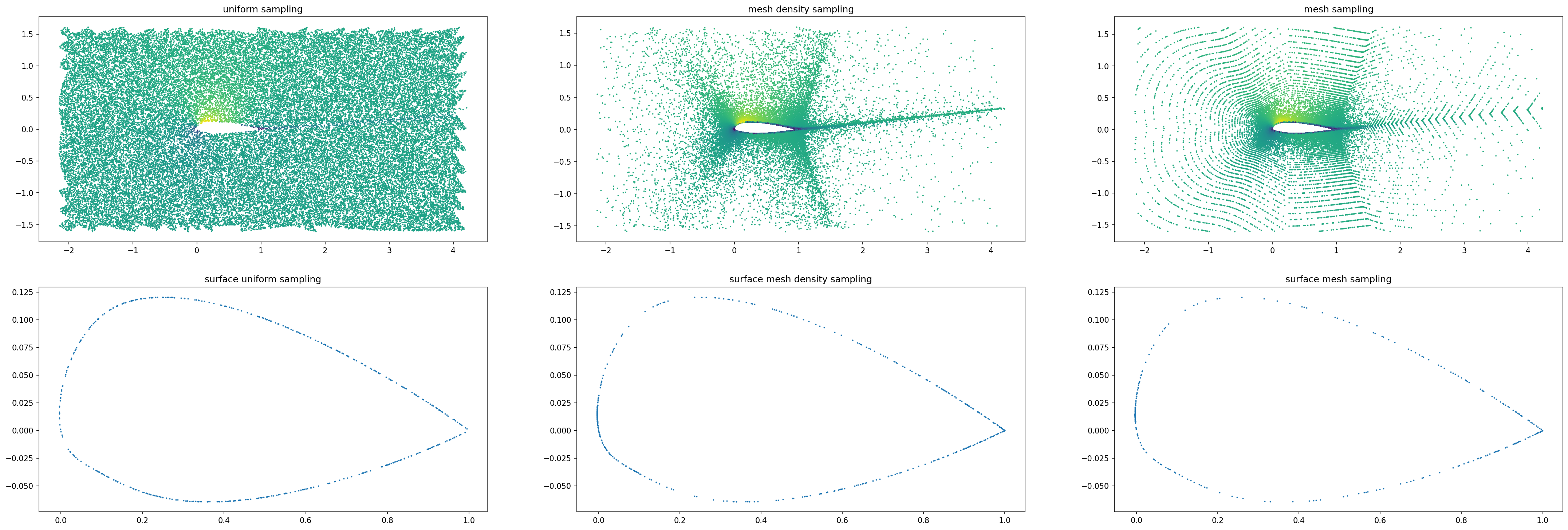
Sampling methods are available allowing to potentially free the constrainte of the mesh structure:

airfrans.Simulation.sampling_volume allows sampling from two different densities on the internal mesh domain
airfrans.Simulation.sampling_surface allows sampling from two different densities on the airfoil mesh domain
airfrans.Simulation.sampling_mesh allows the sampling of nodes in the internal mesh

seed = 0

sampling_volume_uniform = simulation.sampling_volume(seed, 50000, density = 'uniform')
sampling_volume_mesh = simulation.sampling_volume(seed, 50000, density = 'mesh_density')

sampling_surface_uniform = simulation.sampling_surface(seed, 500, density = 'uniform')
sampling_surface_mesh = simulation.sampling_surface(seed, 500, density = 'mesh_density')

sampling_mesh = simulation.sampling_mesh(seed, 50000)
sampling_mesh_surface = sampling_mesh[sampling_mesh[:, 2].astype('bool')]

fig, ax = plt.subplots(2, 3, figsize = (36, 12))
ax[0, 0].scatter(sampling_volume_uniform[:, 0], sampling_volume_uniform[:, 1], c = sampling_volume_uniform[:, 3], s = 0.75)
ax[0, 1].scatter(sampling_volume_mesh[:, 0], sampling_volume_mesh[:, 1], c = sampling_volume_mesh[:, 3], s = 0.75)
ax[0, 2].scatter(sampling_mesh[:, 0], sampling_mesh[:, 1], c = sampling_mesh[:, 8], s = 0.75)
ax[1, 0].scatter(sampling_surface_uniform[:, 0], sampling_surface_uniform[:, 1], s = 0.75)
ax[1, 1].scatter(sampling_surface_mesh[:, 0], sampling_surface_mesh[:, 1], s = 0.75)
ax[1, 2].scatter(sampling_mesh_surface[:, 0], sampling_mesh_surface[:, 1], s = 0.75)
...

You can also directly compute the wall shear stress and the force coefficient with the class attributes or the reference simulation:

simulation.velocity = np.zeros_like(simulation.velocity)
simulation.pressure = np.zeros_like(simulation.pressure)

print(simulation.force())
>> (array([0., 0.]), array([-0., -0.]), array([0., 0.]))

print(simulation.force(reference = True))
>> (array([-79.15, 907.93]), array([-87.92, 906.80]), array([8.78, 1.14]))

print(simulation.force_coefficient())
>> ((0.0, 0.0, 0.0), (0.0, 0.0, 0.0))

print(simulation.force_coefficient(reference = True))
>> ((0.0134, 0.0056, 0.0079), (0.8099, 0.8097, 0.0002))

Some classical metrics between the attributes fields/forces and the reference fields/forces, for example the mean squared error:

print(simulation.mean_squared_error())
>> array([1100.53, 228.03, 227577.73, 0.])

simulation.reset()
print(simulation.mean_squared_error())
>> array([0., 0., 0., 0.])

Finally, you can save new .vtu and .vtp files with the fields given in attributes of the class:

simulation.save(root = SAVING_PATH)